Localization and Path Tracing for Three-Dimensional Image Acquisition

Problem Statement

The goal of this project is to use an Inertial Measurement Unit (IMU) which is placed along with a general commodity phone which is used by a user to capture images of a target from various angles/positions, such that they can capture all the images of the entire target.

This data will then be used to render a 3D plot where the viewer can trace the path taken to capture all the images and highlight the instances at which the images were clicked along with the orientation of the camera.

Software Stack and External Libraries Used

The complete project was developed with Python. Minimal external libraries were used. This was done to implement the entire project from scratch and understand the details of each component of the project. The external libraries used are:

OpenGL and PyGame: These libraries are used to draw the 3D plot which was discussed in the fifth step of the pipeline.
Matplotlib: Matplotlib was used to visualize the position in 3D space during the testing phase for calculating the position data.
NumPy: NumPy arrays are very powerful and are very fast for computation compared to primitive arrays. These were particularly helpful in the prototyping and testing phase. These are still used in the final code for reading CSV files and Quaternion calculations, due to their faster calculation speeds.
Pandas: Pandas dataframe are used to correlate between the time of image capture and the position of the body. Initially, primitive arrays were used, but due to slower speed, this functionality was migrated to Pandas, as querying is faster due to its relational nature.

Methodology and Results

A general commodity mobile phone was used to capture images of a subject.

Once the images were captured, a pipeline is executed, which comprises 5 steps:

Raw data from the IMU is collected using a WIT Motion IMU to an Excel sheet.
The data from the IMU is used to calculate the position and rotation.
Metadata such as image name, timestamp, etc are extracted from the images.
Correlation between the captured image timestamp and IMU readings are drawn.
A Three-Dimentional plot is generated which displays the path taken by the user to capture the images.

Details about each of these steps are explained below.

Collecting raw data from IMU

An IMU gives raw accelerometer, magnetometer, and gyroscope values for the 3 axes.

The IMU used in this project is a WIT Motion sensor. The WIT Motion sensor at its heart has an MPU-9250 IMU, a MEMS motion tracking sensor with 9-DoF (accelerometer, magnetometer, and gyroscope across 3 axes). The end of life for this sensor was announced in 2018 and is replaced by ICM-20948, which is more accurate and consumes lesser power. Nonetheless, MPU-6250 is still accurate and is sufficient for the project.

Manufacturers of the WIT Motion sensor have provided a User Interface for Windows and Mac using which data points were recorded from the IMU using Bluetooth to a CSV file.

One advantage of using this bundled hardware was that the software records the timestamp of each reading.

A script was developed which calculates the time difference between each timestamp and adds this column to the CSV file created.

Calculating the attitude and position of the body using IMU

This was the most crucial part of the project which required a lot of literature survey and research.

The IMU gives raw accelerometer, magnetometer, and gyroscope values across the 3 axes.

In theory, the position of the sensor can be obtained by integrating the acceleration obtained from the IMU twice after subtracting the gravity. When done over a series of data points, we can map the path.

However, this does not work in practice as even the smallest error gets blown up during the double integration process. Moreover, a lot of errors get accumulated due to potential drift and noise generated by the IMU.

Additionally, IMUs do not provide an absolute reference frame for the position, therefore, any initial errors or drift in the measurement will accumulate over time and cause the calculated position to diverge from the true position.

As part of the problem statement, the attitude of the body (Rotation – Roll, Pitch, Yaw) needed to be calculated too.

To get the relative position and attitude of the body, the following techniques were implemented and evaluated, all the source codes are available on GitHub.

Double Integration:

The position of the body is determined by integrating the acceleration once, to obtain the velocity. The velocity obtained is integrated again, to obtain the relative position of the body.

velocity_t = velocity_t-1 + acceleration_t * dt

position_t = position_t-1 + velocity_t * dt

Complementary Filter (Accelerometer and Gyroscope)

The IMU's roll, pitch, and yaw angles were determined using a complementary filter. The function takes three input arguments - acceleration, gyroscope, and time.

The function retrieves acceleration and gyroscope readings and computes the time interval dt. Using the acceleration readings, the roll, pitch, and yaw angles are calculated using the following trigonometric functions:

roll = math.atan2(accel_y, accel_z)

pitch = math.atan2(-accel_x, math.sqrt(accel_y ** 2 + accel_z ** 2))

yaw = math.atan2(accel_y, math.sqrt(accel_x ** 2 + accel_z ** 2))

The change in roll, pitch, and yaw angles from the gyroscope readings are then calculated by multiplying the gyroscope readings by the time interval dt.

The complementary filter is then applied to fuse the gyroscope and accelerometer readings to get accurate roll, pitch, and yaw values. The complementary filter is a weighted average of the gyroscope and accelerometer readings. The weights are set by two constants ALPHA and BETA which are determined experimentally. In all the functions, the yaw angle is normalized, to maintain a range of (-180, 180).

Complementary Filter (Accelerometer, Gyroscope, and Magnetometer)

The general idea behind this algorithm is an extension of the previous one. The main difference is the inclusion of the magnetometer readings to obtain a more accurate measurement of the yaw angle.

Using the formula discussed in the previous section, calculate the roll and pitch angles from the accelerometer readings.

roll_acc = math.atan2(accel_y, accel_z)

pitch_acc = math.atan2(-accel_x, math.sqrt(accel_y ** 2 + accel_z ** 2))

This function provides a more accurate measurement of the yaw angle by compensating for the effects of the roll and pitch angles on the magnetometer readings.

yaw = math.atan2(mag_z*math.sin(roll_acc) - mag_y*math.cos(roll_acc), mag_x * math.cos(pitch_acc) + (math.sin(pitch_acc) * (mag_y*math.sin(roll_acc) + mag_z * math.cos(roll_acc))))

This value is fused with the yaw value obtained from the gyroscope readings, and a more accurate roll, pitch, and yaw value is obtained.

Quaternion-based sensor Fusion

This approach uses Quaternions to describe the orientation of the body in a 3D space. Quaternions are represented as 4D vectors.

Quaternions are more computationally efficient than Euler angles.

Quaternions also avoid the problem of gimbal lock. Gimbal lock occurs when two or more of the axes used to define an object's orientation become aligned, causing a loss of one degree of freedom and making it impossible to represent certain orientations using Euler angles. Quaternions do not suffer from this problem.

The algorithm takes accelerometer and magnetometer as input along with quaternion values that were computed by the WIT Motion sensor.

Here is the approach used:

We loop through each datapoint and
Calculate the expected acceleration in the body frame using the quaternion, gravity vector, and accelerometer measurement.
We then calculate the error in the accelerometer measurement and apply a correction to the quaternion using the accelerometer data.
We then calculate the expected magnetic field in the body frame using the quaternion and magnetometer measurement.
This is followed by calculating the error in the magnetometer measurement assuming the expected magnetic field is [1.0, 0.0, 0.0], and a correction to the quaternion is applied using the magnetometer data.
After updating the quaternion, we calculate the position of the object by integrating the velocity obtained from linear acceleration, which is obtained by multiplying the acceleration quaternion by the rotation matrix.
The roll, pitch, and yaw angles are also obtained using the rotation matrix (quaternion).

Quaternion-based sensor Fusion with calibration

A constant bias was observed in the IMU data. Therefore, this function, which is an extension of the previous section was developed to eliminate the bias.

More details about bias removal are discussed in the ‘Bias Removal’ section of the report.

This is an extension of the above approach where a constant bias was removed from the IMU readings.

Sensor Fusion with Madgwick Filter

This solution gave the best results among all other approaches, as I incorporated all the prior learnings with learnings from other scholars. Madgwick Filter was developed by Sebastian Madgwick in 2010 and uses a gradient descent approach to optimize a quaternion representing the orientation of the object in space. It incorporates IMU measurements to estimate the quaternion which minimizes the error between the predicted and measured values. The filter is computationally efficient and can provide accurate orientation estimates even in the presence of magnetic disturbances and other environmental factors.

The proposed solution follows the below approach:

The quaternion is initialized with identity quaternion (No rotation). A loop is executed across all the data points with the below operations.
Static Biases are removed from the accelerometer, gyroscope, and magnetometer readings. They are then normalized.
Objective Function: The algorithm computes an objective function f based on the current orientation estimates of the quaternion vector and the normalized accelerometer and magnetometer measurements. This function represents the error between the estimated and measured values (start of Madgwick).
Jacobian matrix: The Jacobian matrix is calculated which represents the rate of change of the objective function with respect to the quaternion components.
Gradient Descent: The algorithm computes the gradient of the objective function by multiplying the transpose of the Jacobian matrix j.T with the objective function f. The gradient is then normalized and multiplied by the tuning parameter beta.
This is followed by taking the derivative of quaternion using the gyroscope measurements and the computed gradient. This represents the rate of change of the quaternion over time.
Value of quaternion is updated by integrating the results obtained from the above (end of Madgwick).
Effect of gravity is eliminated from the raw accelerometer readings. It takes raw accelerometer measurements and the current orientation quaternion, then computes world frame representations of gravity and accelerometer data. It subtracts the gravity component from the accelerometer data, returning linear acceleration without gravity.
Velocity and Position are obtained by integrating the acceleration.
Lastly, Rotation Data is obtained using trigonometry on the quaternion data.

Image Metadata Extraction

When an image is captured, the camera applications record some metadata too. This data formatting is generally common across all cameras and is known as EXIF data (exchangeable image file format). The function get_image_exif_data() extracts metadata for all the images using the Python Imaging Library.

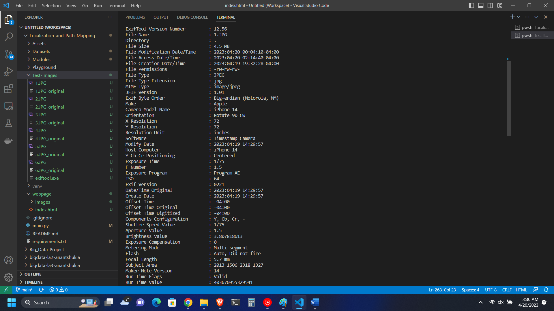
Figure 1: EXIF data of a sample image.

Correlation between captured image timestamp and IMU Data

The function correlate_timestamp_with_position() correlates the timestamp of each image with the corresponding timestamp of IMU readings to assign position and rotation data to each image. This data is combined into a common data structure and used in the subsequent section to draw the 3D plot on OpenGL. Generally, stock camera apps give minute-level accuracy of when the image was captured. However, some applications exist on app stores, which record millisecond timestamps. We will require millisecond accuracy to accurately plot the location of image with the path taken.

Three-Dimensional Plot Generation

Python's binding with OpenGL is used to generate a 3D plot with which the user can visualize the path taken to capture the images along with the points. Additionally, the plot cycles through all the points where the images were captured and displays the orientation of the camera for all the images.

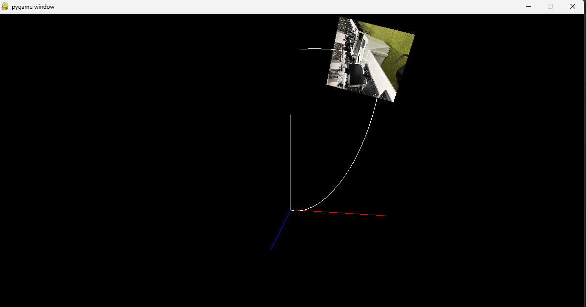
Figure 2: 3D Plot on OpenGL

3. Challenges

Due to several challenges, research on this topic is often dropped or left incomplete. This section discusses the challenges observed.

3.1. Constant Bias Observed in IMU Data

Constant bias or static bias is a fixed offset error that can accumulate over time and lead to significant errors in calculated measurements. To tackle this, the IMU is kept on a stable surface for ~10 seconds. An average of these readings is calculated, and this average is subtracted from each data point to eliminate the constant bias. F_calib= F_raw-bias This helped reduce a constant Z-axis bias but could not eliminate it, there is a significant Z-axis increase over time.

Noise in magnetometer values

The Magnetometer sensor is very susceptible to interference. When trying to capture images with the IMU attached to the phone, the IMU readings were very noisy resulting in errors of a huge margin. To mitigate this, IMU and the phone were supposed to be kept far apart, making sure that the IMU does not come near other electrical and ferromagnetic materials. But, while this helped in getting accurate position values for the user, this resulted in getting incorrect rotation values for the camera, as the IMU was not attached to the phone.

3.3. Drift generated by IMU

The IMUs' orientation is obtained by integrating the angular velocity measured by the reading obtained using the gyroscopes. This gives us immediate orientation changes but leads to a drift of the estimated orientation over time. This drift in the gyroscope is a result of a low-frequency variable called bias instability and in the accelerometer by a high-frequency variable called angular random walk. This leads to a lot of errors obtained over time.

Mitigating the drift led to a lot of research. In the future improvements of the project, research into further improving the Madgwick Filter and obtaining better gain values can be done, for further improvement, Kalman Filtering or Extended Kalman Filter can be used to improve accuracy.

3.4. Latency between sensor and computer

When the user tries to capture images of the target even 4-5 meters away from the computer, data points were observed to be sent once in 1-3 seconds, which increases error.

3.5. Research and validation

Due to the complicated nature of the topic, a lot of research was required while implementing the solution. This required an understanding of rotation matrices, quaternions, trigonometry math, and knowledge about the sensor. This resulted in a lot of time being spent just to validate whether the implementation was correct. Or validating whether an error is induced by incorrect IMU readings.

Results

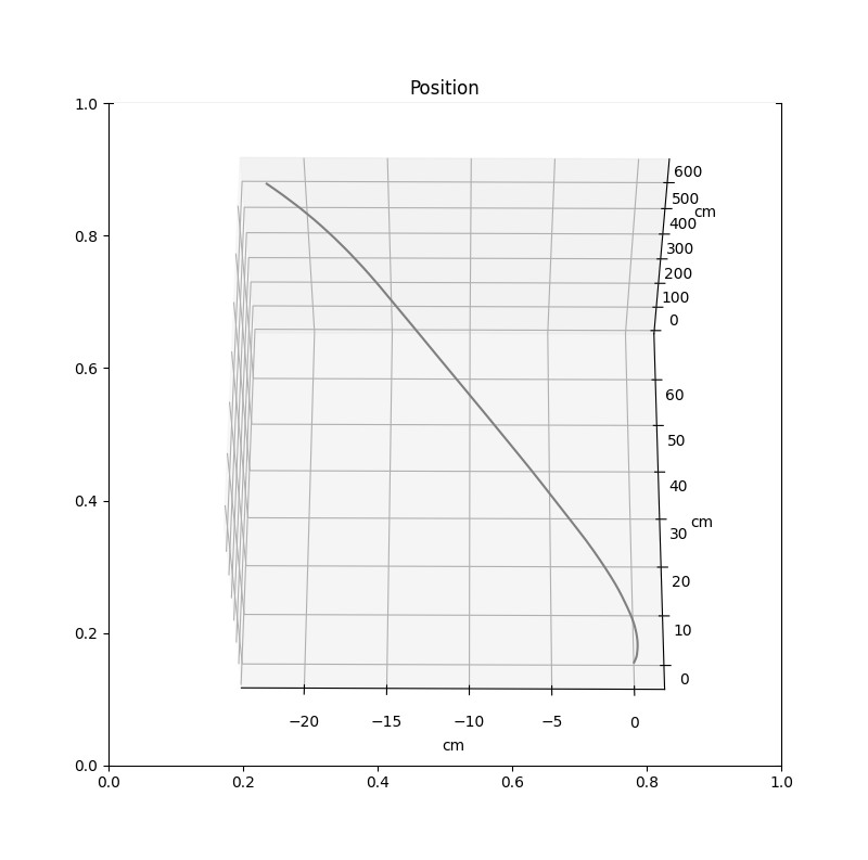
Figure 3: Position when IMU was moved in a straight line.

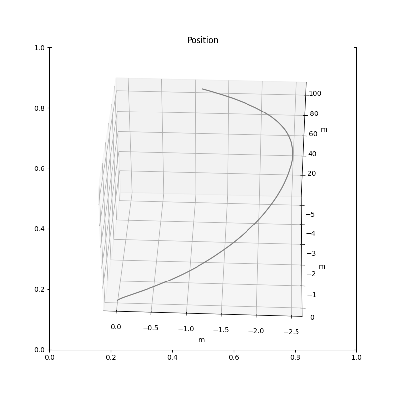
Figure 4: Position when IMU was moved in an ellipse along the target.

Video: Demo of the Visualization.